Professor Sheryl Grace
Dept. of Aerospace and Mechanical Engineering
Boston University
Research Assistant: Brad Mahoney
Columbia University
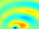
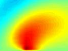
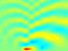
This visualization demonstrates the unsteady pressure field resulting from the interaction of a gust and a flat-plate airfoil. Shown are comparisons of the effects of altering the Mach Number and reduced Frequency.
An unsteady pressure field (i.e. “acoustic field”) is created when an unsteady, subsonic, compressible flow passes a flat-plate airfoil. In this analysis it is assumed that the unsteady field quantities are small compared to the mean quantities. The unsteady disturbance simulated here is a vortical gust. This is a basic model for an airfoil chopping through what can be thought of as isotropic turbulence.
These images represent the solution obtained by solving the linearized Euler equations. This direct calculation of sound is performed in two steps. First, the incoming flow must be characterized and its influence on the airfoil calculated. This entails measuring the Mach number M of the flow. Mach number is the ratio of the flow speed to the speed of sound for the fluid. The main spectral structure of the vorticity must also be given. We assume that there are discrete frequencies which carry most of the turbulent energy and consider each frequency separately. The parameter which quantifies the frequency is the reduced frequency
Here f is the frequency, c is the airfoil chordlength, and U is the mean-flow speed. The flat-plate airfoil response is characterized by the unsteady pressure jump across the airfoil from leading edge to trailing edge. The unsteady pressure jump is calculated by solving an integral equation numerically using a collocation technique. This code was written in FORTRAN several years ago at The University of Notre Dame.
The second step is accomplished by applying Green’s theorem to a manipulated version of the governing equations. Subsequently, a rather “simple” integration of the unsteady pressure jump along the airfoil (known from step one) multiplied by the appropriate Green’s function gives the corresponding unsteady pressure at any location around the airfoil. This is also know as the Kirchhoff method for calculating aeroacoustic results.
The video depicts the unsteady pressure fields (acoustic fields) that arise when various combinations of flow speeds and gust frequencies are simulated. The flat-plate airfoil lies on the bottom edge of the picture between -1 and 1. For this problem, the acoustic field below the airfoil is symmetric to the one above, so it is not shown. The complex radiation patterns are easily visible by colormapping the values of the nondimensional unsteady pressure.
The visualization and the numerical integration codes for the second part were done by Brad Mahoney.

Video Sequence
Mach Number=.3
Reduced Frequency=3
Video Sequence
Mach Number=.3
Reduced Frequency=7
Video Sequence
Mach Number=.5
Reduced Frequency=1
Video Sequence
Mach Number=.8
Reduced Frequency=1
Hardware: IBM RS6000.
Software: FORTRAN, MATLAB.
Video Production and Matlab assistance: Kathleen Curry, Scientific Computing and Visualization Group, Boston University.
Acknowledgments: Brad Mahoney’s work was done while he was a participant in the Boston University Research Experience for Undergraduates Program sponsored by the National Science Foundation.